9.2.3.   Genetic Algorithm Framework

The genetic algorithm framework introduced in chapter 7 was applied to the calibration data set with 100 parallel runs of the GA. Each GA run evaluated 50 populations using about 60 generations whereas the stopping criterion was set to a convergence of the standard deviation of the genes below 0.04. The parameter a of the fitness function was set to 0.9 resulting in the selection of approximately 6 variables per single GA.

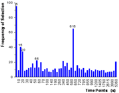
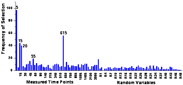
The ranking of the variables after the first step is shown in figure 63. In the second step, these variables entered the model according to their rank until the prediction of the test data did not improve significantly. In contrast to chapter 7, a Kruskal-Wallis non-parametric test (p<0.05) was used to test the significance of improvement for the 20-fold random subsampling procedure (see section 10.2 for a detailed discussion). The iterative procedure stopped after the addition of 5 variables with the selection of the time points 5 s, 15 s, 25 s, 55 s and 615 s, which are labeled in figure 63.

figure 63:  Frequency of the variables selected in the first step of the genetic algorithm framework.

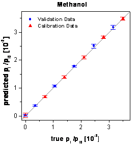
The optimized networks using only these 5 variables instead of all 50 variables show the best predictions of the external validation data (see table 6). Additionally no gap is visible between the predictions of the calibration data and the validation data. The corresponding true-predicted plots are shown in figure 64. The signals of 3 times 18 reproduced measurements, which were spread over the complete concentration range of the samples of the mixtures, show a relative standard deviation of 4.6 %. These inaccuracies of the signals are caused by the noise of the spectrometer, inaccuracies of the gas mixing station and fluctuations of the measuring temperature. The rather small increase of the mean relative RMSE in the concentration domain (5.8% versus 4.6%) after the data analysis demonstrates the calibration power of the genetic algorithm framework.

figure 64:  Predictions of the calibration and validation data by the neural networks optimized by the genetic algorithm framework.

The 5 time points selected by the framework (5 s, 15 s, 25 s, 55 s and 615 s) can be analyzed in more detail when looking at the sensor response plots (figure 16). The response surface of methanol shows that after 5 seconds the response has practically reached the plateau of the highest sensor signals whereas ethanol and 1-propanol hardly show any sensor signal. The same applies to the 615 s signal, which is situated 15 seconds after the end of exposure to analyte: Methanol has already desorbed whereas the sensor response of ethanol is still very high and 1-propanol shows practically no decrease of the sensor signal. Thus, the 5 s signal represents the concentration of methanol, whereas the 615 s signal represents the sum of the concentrations of ethanol and propanol. Large parts of the variance of the sensor signals after 15 and 25 seconds can be identified with ethanol since the signal of methanol has already reached the plateau and 1-propanol attributes negligibly to the total signal. On the other hand, the variance of the sensor signal at 55 seconds can be mainly ascribed to 1-propanol whereby the sensor response of methanol has completely and the sensor response of ethanol has nearly reached equilibrium. In summary, it may be said that all 5 time points selected by the algorithm can be associated with the characteristic sensor responses of the pure analytes and consequently make sense in a chemical respect. Another benefit from the variable selection results from the direct relation of the variables with the time needed for the analysis. Only information during 55 seconds of exposure to analyte and 15 seconds after the end of exposure is evaluated. Thus, it should be enough to reduce the time of exposure to analyte to 55 seconds and to record the sensor responses during 70 seconds. This would dramatically reduce the analysis time.

Similar to section 7.3, a randomization test was performed to test the reproducibility and robustness of the variable selection and of the calibration. For this test, 50 uniformly distributed autoscaled random variables were added to the set of 50 original time points. The genetic algorithm framework was used for this extended data set the same way as described before except of increasing the population size to 100 resulting in about 110 generations until the convergence criterion was reached and except of setting the parameter a to "1", which resulted in approximately 6 variables being selected in single runs of the GA. The ranking of the variables after the first step of the algorithm is shown in figure 65.

figure 65:  Ranking of variables for 50 time points and for 50 additional random variables.

It is obvious that all random time points are ranked very low and no random variables can be found among the most important 27 time points. Similar to section 7.3 the parallel runs of multiple GA prevented the selection of randomly correlated variables whereas single runs of the GA selected random variables. The left side of figure 65 looks very similar to figure 63 demonstrating the reproducibility of the ranking of meaningful variables. The top 5 time points are ranked similarly to the algorithm applied to the original data. Consequently, the same 5 variables are selected in the second step of the algorithm demonstrating the reproducibility of the selection of the variables by the genetic algorithm framework.