For the
application of the growing neural net algorithm, the calibration data set was
split into a training (80 %) and a monitor (20%) subset by a random subsampling
procedure (see section 2.4).
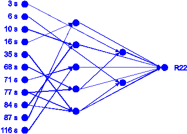
Using the stopping criterion of 0.1% minimal error decrease the growing network
algorithm built the network for R22 shown in figure
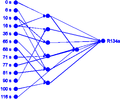
50 with 11 input neurons, 22 links and 7 hidden neurons organized in 2 hidden
layers. For R134a the network consisted of 13 input neurons, 23 links and 7
hidden neurons organized in 2 hidden layers shown in figure
51.
figure 50: Neural network built
by the first run of the growing neural network algorithm for R22.
figure 51: Neural network built
by the first run of the growing neural network algorithm for R134a.
These
network topologies were trained using the complete calibration data set and
then predicted the concentrations of the external validation data. According
to table 4 in section
8.5, the grown neural networks predicted the external validation data not
used for the network growing process significantly better than non-optimized
static neural networks and no significant gap between the predictions of the
calibration and validation data is visible.
Yet,
similar to the application of single run genetic algorithms for the optimization
of neural networks (see section 2.8.9), the topology
of the grown networks depends highly on the partitioning of the data set. A
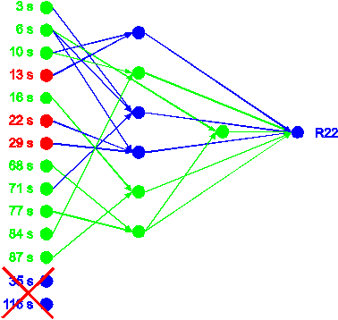
second run of the algorithm with differently subsampled training and monitor
data subsets resulted in other network topologies for both analytes. The network
for R 22 of this second run is shown in figure 52.
Although several substructures, which are printed in green, are equal to the
network shown in figure 50, both networks also show
significant differences, which are printed in blue in figure
52. In principle, these differences of the network topology are not necessarily
bad as for a given set of input variables the approximation of a functional
relationship between the input and the response variables can be performed by
a neural network on nearly uncountable ways. Yet, the selection of different
variables during different runs is by far more problematic. For example, the
second network uses the time points 13 s, 22 s and 29 s instead of 16 s and
116 s as input variables, which are printed in red in figure
52. The selection of different variables irreversibly changes the possibilities
of the functional mapping and significantly influences the quality of calibration.
As can be seen in table 4, the predictions
of the validation and calibration data differ for the nets built during the
different runs whereby the growing neural nets performed generally better for
the validation data than the static neural nets during several runs. Also, the
network of the second run for R134a with 10 input neurons, 18 links and 5 hidden
neurons organized in 1 hidden layer differs significantly from the network of
the first run for R134a in respect to the topology and even worse in respect
to the selected variables.
Similar
to the single runs of genetic algorithms the topology and more important the
selection of the variables are representative for only one partitioning of the
data set into calibration and monitor data set and not for the complete data
set. Analogous to the framework of the genetic algorithms (section
7.2), two frameworks are proposed in the next section to make the variable
selection of the growing neural networks less sensitive to the partitioning
of the data into different subsets and to different random initial weights.
In section 8.4, these two frameworks are applied to the
refrigerant data sets resulting in improved calibrations.
figure 52: Neural network built
by the second run of the growing neural network algorithm for R22. Elements
equal to the network of the first run are printed in green.